Ranking and Rating Systems
Ranking and Rating Systems
When you play an online multiplayer game, how does the system decide which opponent out of the opponent pool to match you with? When you play chess against an opponent and win, how does the system decide how much to change your respective ratings by? These are questions I never thought about until my internship at AICrowd. It turns out these are really interesting problems with complex solutions and real world applications. The problem boils down to estimating the skill distribution of a population in a game, given their performance in some games. We may then the this estimate to match people in future games, or rank them in order of skills. There are various algorithms for this problem, like Elo and TrueSkill. I took an Independent Study on Monte Carlo Markov Chain Sampling last semester at the university. My motivation for exploring these further was to use MCMC techniques to give theoretical bounds on number of rounds of games necessary before the matching becomes ‘good enough’, by formulating the problem in terms of sampling from a markov chain. We can define ‘good enough’ in various ways. It turns out I didn’t end up tackling this problem in specific for various reasons, but I did learn a little about these topics throughout the remainder of the semester. Here I’ll write about some of these concepts, as well as about Elo and TrueSkill. Let’s define some terms first.
- Skill: We can define some scale for a ‘skill’ measure, which would indicate a player’s skill in playing that game. For example, we can take $0$ to indicate a really poor player (beginner at a game), and \(500\) and above to be really good (expert) player. We assume that this is represented by some continuous distribution, like a gaussian.
- Real Skill: This is the player’s real world skill, the skill with which his performance in a game would be determined. This is the skill we want to estimate in our problem.
- Performance: This is a player’s skill in one particular game. This can be different from real skill since there can be a variation to how well a player will perform in each game if he is playing multiple games simultaneously. (She could be tired, hungry or drunk.)
- Estimated Skill: This is an estimate of real skill that our algorithm will determine. We want this to be as close to real skill as possible.
- Round: Each round is one game or match. Two or more players compete, and the outcome is a binary variable determining the winner, or a draw.
- Tournament: A collection of rounds will form a tournament.
Elo rating system
It is a method for calculating the relative skill levels of players in zero-sum games such as chess. It is named after its creator Arpad Elo. It is extensively used in games other than chess as well, with little modification.
In Elo, the skill estimate is considered to be a whole number called the Rating, and the values are updated as the outcomes of more and more games becomes available. Players’ ratings depend on the ratings of their opponents and the results scored against them. The difference in rating between two players determines an estimate for the expected score between them. Players with higher rating have a higher probability of winning a game than a player with lower rating. After each game, rating of players is updated. If a player with higher rating wins, only a few points are transferred from the lower rated player. However if lower rated player wins, then transferred points from a higher rated player are far greater.
If players A and B have ratings \(R_A, R_B\), respectively, then their expected score \(E_A\) and \(E_B\) (the probability of winning) is given as follows:
\[E_A = \frac{1}{1 + 10^{\frac{R_B - R_A}{400}}} = \frac{Q_A}{Q_A + Q_B} \\ E_B = \frac{1}{1 + 10^{\frac{R_A - R_B}{400}}} = \frac{Q_B}{Q_A + Q_B}\]where \(Q_i = 10^{\frac{R_i}{400}}\). The constants 10 and 400 are set such that that for each 400 rating points of advantage over the opponent, the expected score is magnified ten times in comparison to the opponent’s expected score. Now we can use this expected score or the winning probability to update the ratings of the players involved. A simple adjustment is given as follows.
\[R'_A = R_A + K (S_A - E_A) \\ R'_B = R_B + K (S_B - E_B)\]Here, \(R'_i\) is the new rating of the \(i^{th}\) player, \(S_i\) is the score of the \(i^{th}\) player, which can be binary (0-1) values, denoting a loss or a win, or it can be something else. The constant \(K\) here is the called the K-factor, and it denotes the maximum possible rating change in one game. This is because, the maximum difference between expected and actual score can be 1, changing the rating of the players involved by \(K\). We can also use different K-factors for players with varying experience on a platform (i.e., players whose ratings we are more confident on can have a lower K-factor than otherwise.)
There are some drawbacks to Elo, such as it does not apply directly to team games, or games involving more than two players.
Trueskill
TrueSkill is a model based approach to the match making problem, based on the assumption that the skill of a player is an uncertain quantity, and should be modelled using a probability distribution. We’ll try to understand this model here.
Assumptions
As mentioned above, TrueSkill is a model based rating system. Here are the assumptions of the model:
- Each player has a skill value, represented by a continuous variable with a broad Gaussian distribution.
- Each player has a performance value for each game, which varies from game to game such that the average value is equal to the skill of that player. The variation in performance, which is the same for all players, is symmetrically distributed around the mean value and is more likely to be close to the mean than to be far from the mean.
- The player with the higher performance value wins the game.
Now that the skill values are represented as probability distributions, we can use our knowledge of probabilistic graphical models to represent the random variable associated with performance, skill and the game outcomes as a factor graph, and use belief propagation on the graph to update skill values.
Modelling the outcomes of games
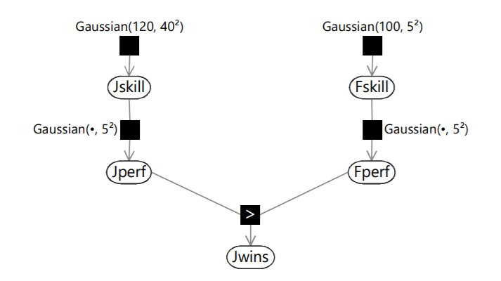
Suppose we have two players, Fred and Jill. They have skills Fskill and Jskill respectively, and their performance is Fperf and Jperf, derived from their skill values. Suppose the Bernoulli variable Jwins denotes the winning or losing of Jill by taking the values true and false respectively. Then, the game can be represented using the following factor graph.

Here we have assumed that the skill of Jill and Fred are represented by Gaussian distributions with means 120 and 100, and variances \(40^2, 5^2\) respectively. A higher variance captures a lower confidence in the estimated skill of a player, and vice versa. The mean for the performance of both players is derived by sampling from the skill distributions, and the variance is a constant \(5^2\). Then, the value of Jwins is given by a simple max function (\(>\) operation).
This model captures the uncertainty in the performance of players, say because of a down day or a bad luck, and also captures the under-confidence in the estimated skills for new players. There is a chance that with some probability, the performance of a player with the higher skill might be lower in a game.
Now if we are given the skill values, we can use the factor graph to find the probabilistic outcome of the game. Or the other way round, given the outcome of a game, we can run inference in order to compute the marginal posterior distributions of the skill variables Jskill and Fskill.
Using belief propagation to update skills
Since the graph has a tree structure, we can use belief propagation to solve this problem.
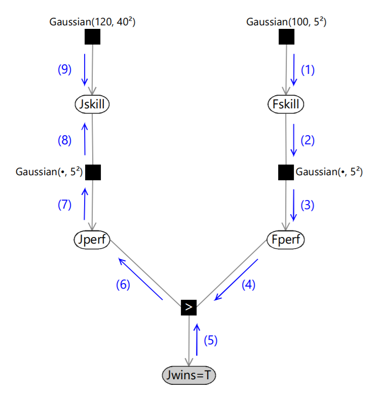
As in the reference, we can take an example to understand this. Suppose Jwins is true, and we want to evaluate the posterior distribution for Jskill. The following figure gives an overview of which messages that need to be evaluated.

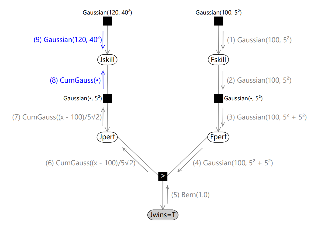
Message (1) is just given by the Gaussian factor itself. Similarly, message (2) is just the product of all incoming messages on other edges of the Fskill node, and since there is only one incoming message this is just copied to the output message. To compute message (3), the belief propagation algorithm tells us to multiply the incoming message (2) by the Gaussian factor and then sum over the variable Fskill. Using convolution, this comes out to be Gaussian(100, \(5^2+5^2\)). Message (4) is just a copy of message (3) as there is only one incoming message to the Fperf node. Message (5) is just a Bernoulli point mass at the value true. Continuing with the algorithm, the final outcome is summarised in the following figure.

The marginal distribution of Jskill is obtained by multiplying messages (8) and (9). Because this is the product of a Gaussian and a cumulative Gaussian the result is an asymmetrical distribution, which is not a Gaussian. This is the posterior distribution for Jskill. We can also pass messages in the opposite direction around the graph to obtain the corresponding posterior distribution for Fskill.
Extending to multiple players – expectation propagation
We have seen how to exactly find posterior distributions for the distributions representing skills of the two players. We can easily extend this to other players, by adding the other games in the same graph, and running belief propagation on the bigger graph one by one. But there is a problem with doing this. Initially, Jskill was a 2 parameter gaussian distribution. After running belief propagation once, we get a distribution which is a product of a gaussian and a cumulative gaussian, and hence has 4 parameters. If we now run belief propagation on a game with another player, we will get another distribution with two cumulative distributions and six parameters.
To get around this problem, we use expectation propagation. We approximate the non-gaussian distributions locally with a gaussian distribution, and we do it in the following manner.
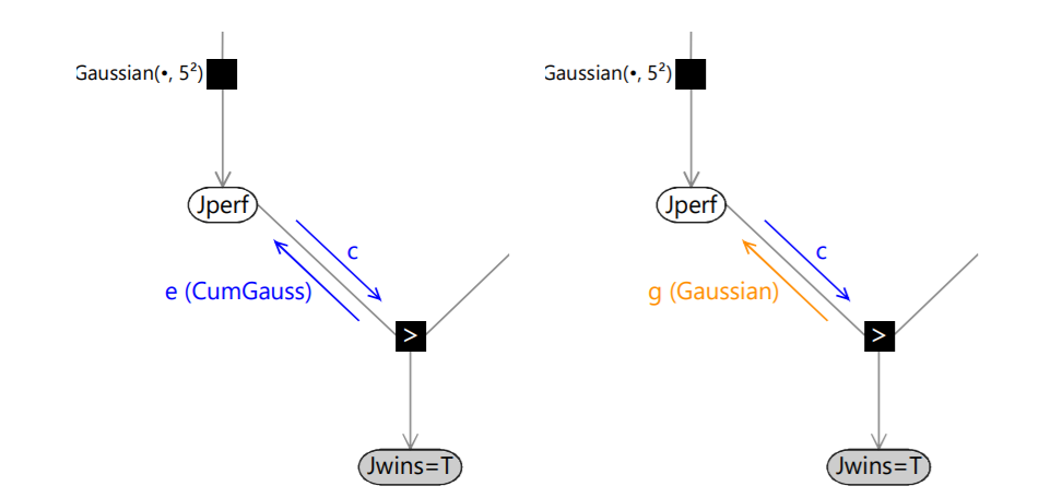
We want to approximate message (6), the cumulative gaussian distribution using a gaussian so as to maximize the accuracy of the marginal distribution of Jperf. We could just replace the Cumulative Gaussian function with a gaussian with the same mean and variance, but that is not possible since the mean and variance of the cumulative gaussian functions are undefined (as \(x \rightarrow \infty\), value of the cumulative gaussian function approaches 1.) We get around this problem by using a ‘context’, which is the downward message on the same edge as the message (6). Let \(e\) denote the exact message (6), \(c\) denote the downward ‘context’ message, and \(g\) denote our desired Gaussian approximation to message \(e\). We use
\[cg = Proj(ce)\]where Proj() is the projection, and represents the process of replacing a non-gaussian distribution with a Gaussian having the same mean and variance. This can be viewed as projecting the exact message onto the ‘nearest’ message within the family of Gaussian distributions. We can now compute \(g\) exactly. This is because the product \(ce\) gives a distribution with finite mean and variance.

This approach of using an incoming message to provide the context in which to approximate the corresponding outgoing message is known as expectation propagation (or EP). With this technique, we can always locally approximate the non-gaussian messages by a gaussian. And we also know that the product of two gaussian distribution is a gaussian. Hence, we now have a posterior distribution which is also a gaussian with 2 parameters, thus is of the same form as the prior. Therefore, we can now easily run the algorithm multiple times without blowing up the parameters in our distribution.
The beauty of this model is that now we can easily add more players to the graph and extend it to work for team games, multi player games, and also handle draws.
Acknowledgement
I thank my friend Athreya Chandramouli for spending hours with me on calls where we tried to understand these topics.